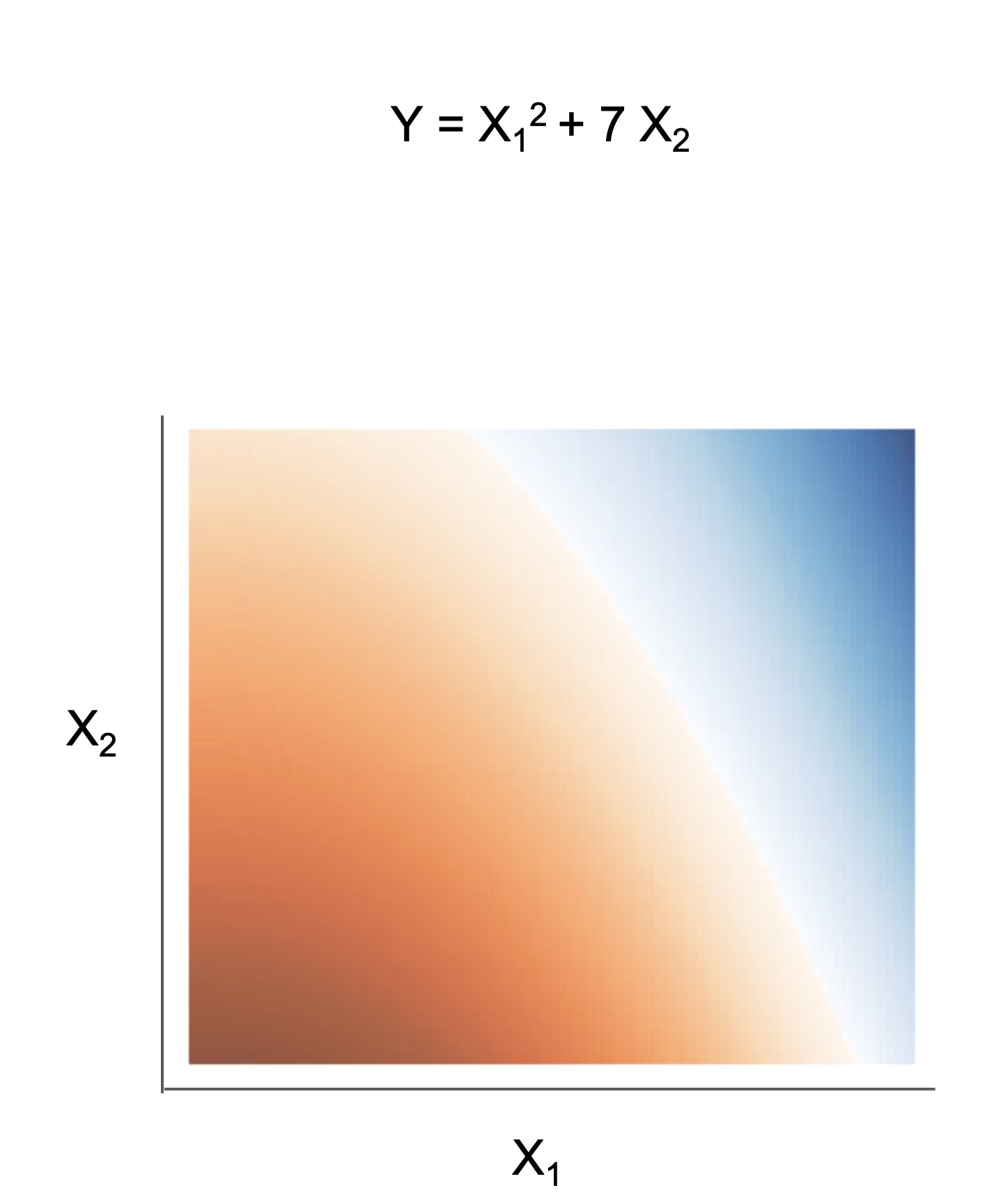
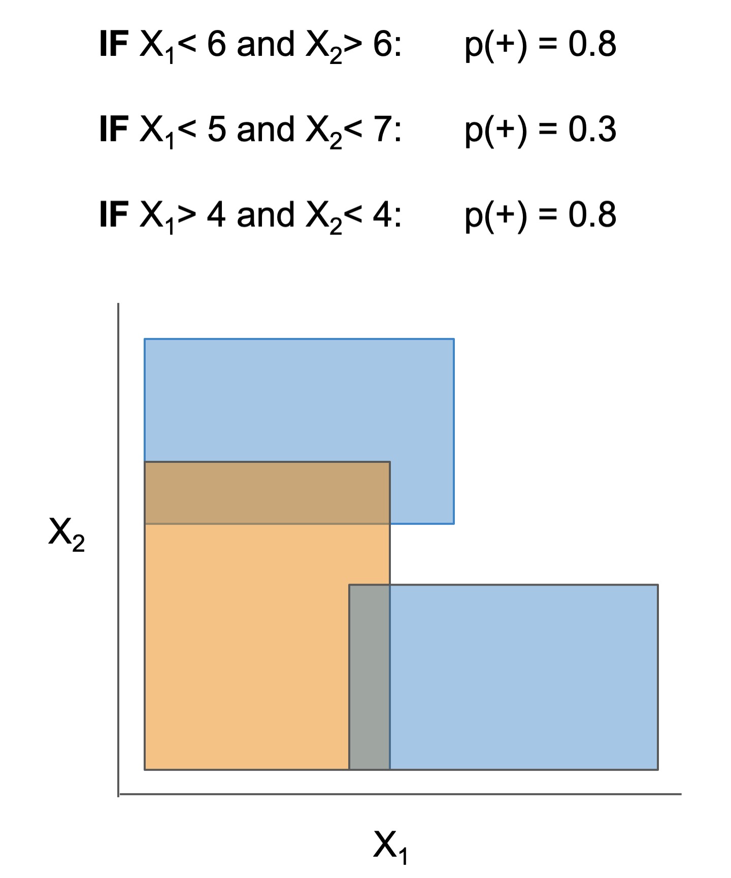
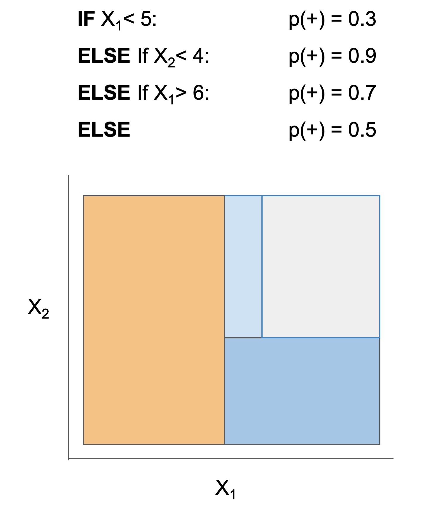
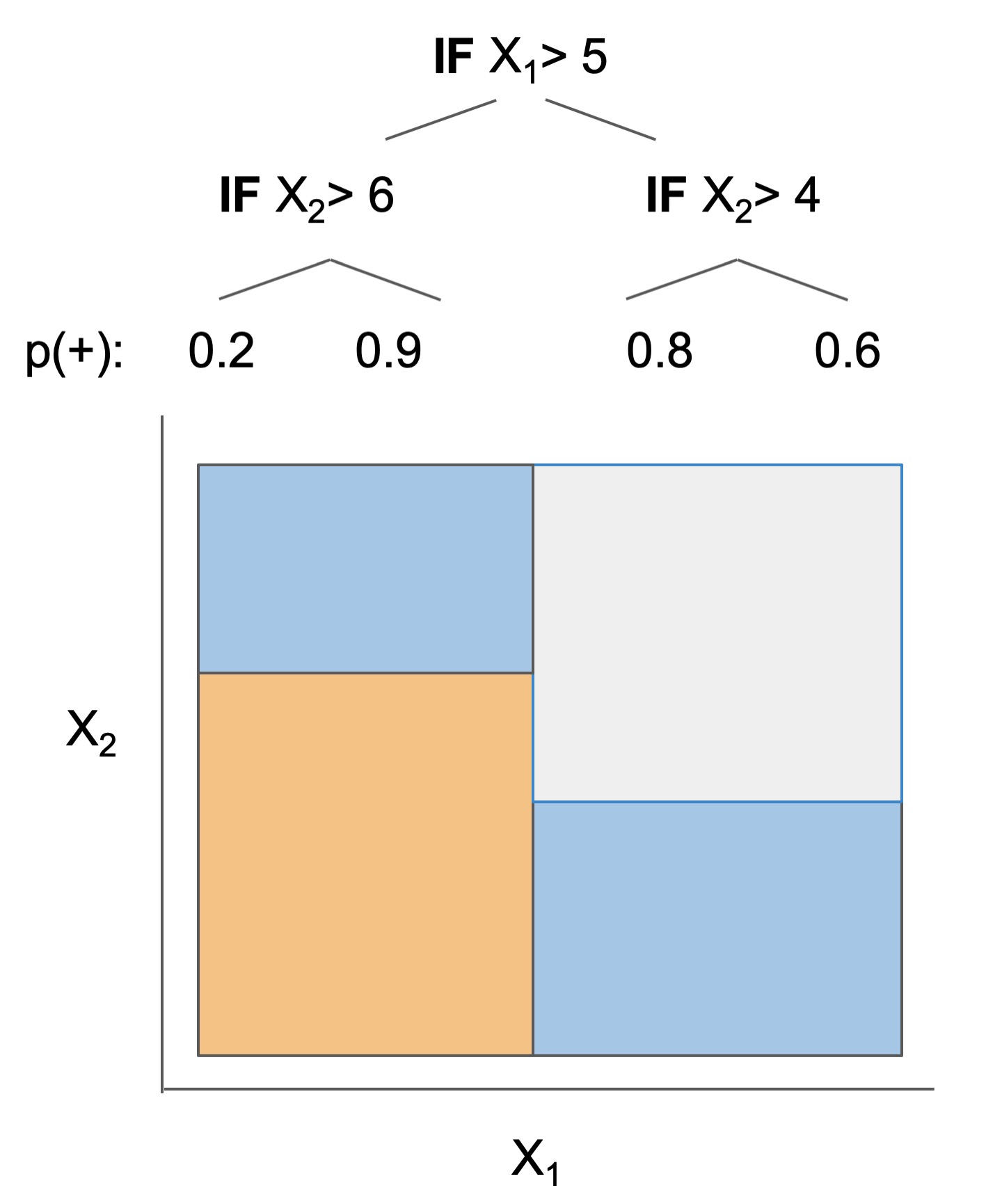
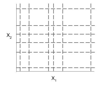
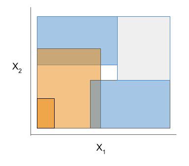
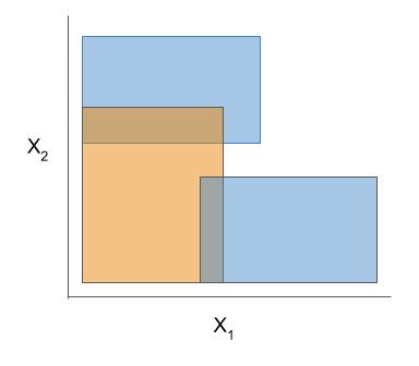
Module imodels.tests.notebooks.imodels_demo

Expand source code
# ---
# jupyter:
#   jupytext:
#     formats: ipynb,../imodels/tests/notebooks//py:percent
#     text_representation:
#       extension: .py
#       format_name: percent
#       format_version: '1.3'
#       jupytext_version: 1.11.1
#   kernelspec:
#     display_name: Python 3
#     language: python
#     name: python3
# ---

# %% pycharm={"is_executing": false}
# %load_ext autoreload
# %autoreload 2
import os

import matplotlib.pyplot as plt
import numpy as np

np.random.seed(13)
from sklearn.datasets import fetch_openml
from sklearn.model_selection import train_test_split
from sklearn.tree import plot_tree, DecisionTreeClassifier
from sklearn import metrics
from scipy.io.arff import loadarff

# installable with: `pip install imodels`
from imodels import SLIMRegressor, BayesianRuleListClassifier, RuleFitRegressor, GreedyRuleListClassifier
from imodels import SLIMClassifier, OneRClassifier, BoostedRulesClassifier

# change working directory to project root
if os.getcwd().split('/')[-1] != 'imodels':
    os.chdir('..')


def get_ames_data():
    housing = fetch_openml(name="house_prices", as_frame=True)
    housing_target = housing['target'].values
    housing_data_numeric = housing['data'].select_dtypes('number').drop(columns=['Id']).dropna(axis=1)
    feature_names = housing_data_numeric.columns.values
    X_train_reg, X_test_reg, y_train_reg, y_test_reg = train_test_split(
        housing_data_numeric.values, housing_target, test_size=0.75)
    return X_train_reg, X_test_reg, y_train_reg, y_test_reg, feature_names
    

def get_diabetes_data():
    '''load (classification) data on diabetes
    '''
    data = loadarff("imodels/tests/test_data/diabetes.arff")
    data_np = np.array(list(map(lambda x: np.array(list(x)), data[0])))
    X = data_np[:, :-1].astype('float32')
    y_text = data_np[:, -1].astype('str')
    y = (y_text == 'tested_positive').astype(int)  # labels 0-1
    X_train, X_test, y_train, y_test = train_test_split(X, y, test_size=0.75)  # split
    feature_names = ["#Pregnant", "Glucose concentration test", "Blood pressure(mmHg)",
                     "Triceps skin fold thickness(mm)",
                     "2-Hour serum insulin (mu U/ml)", "Body mass index", "Diabetes pedigree function", "Age (years)"]
    return X_train, X_test, y_train, y_test, feature_names


def viz_classification_preds(probs, y_test):
    '''look at prediction breakdown
    '''
    plt.subplot(121)
    plt.hist(probs[:, 1][y_test == 0], label='Class 0')
    plt.hist(probs[:, 1][y_test == 1], label='Class 1', alpha=0.8)
    plt.ylabel('Count')
    plt.xlabel('Predicted probability of class 1')
    plt.legend()

    plt.subplot(122)
    preds = np.argmax(probs, axis=1)
    plt.title('ROC curve')
    fpr, tpr, thresholds = metrics.roc_curve(y_test, preds)
    plt.xlabel('False positive rate')
    plt.ylabel('True positive rate')
    plt.plot(fpr, tpr)
    plt.tight_layout()
    plt.show()

if __name__ == '__main__':
    X_train_reg, X_test_reg, y_train_reg, y_test_reg, feat_names_reg = get_ames_data()
    X_train, X_test, y_train, y_test, feat_names = get_diabetes_data()

    # load some data
    print('regression data', X_train_reg.shape, 'classification data', X_train.shape)

    # %% [markdown]
    # # rule sets
    # Rule sets are models that create a set of (potentially overlapping) rules.

    # %% [markdown]
    # ### rulefit

    # %% pycharm={"is_executing": false}
    # fit a rulefit model
    rulefit = RuleFitRegressor(max_rules=10)
    rulefit.fit(X_train_reg, y_train_reg, feature_names=feat_names_reg)

    # get test performance
    preds = rulefit.predict(X_test_reg)
    print(f'test r2: {metrics.r2_score(y_test_reg, preds):0.2f}')

    # inspect and print the rules
    rules = rulefit.get_rules()
    rules = rules[rules.coef != 0].sort_values("support", ascending=False)

    # 'rule' is how the feature is constructed
    # 'coef' is its weight in the final linear model
    # 'support' is the fraction of points it applies to
    rules[['rule', 'coef', 'support']].style.background_gradient(cmap='viridis')

    # %% [markdown]
    # ## boosted stumps

    # %%
    # fit boosted stumps
    brc = BoostedRulesClassifier(n_estimators=10)
    brc.fit(X_train, y_train, feature_names=feat_names)

    print(brc)

    # look at performance
    probs = brc.predict_proba(X_test)
    viz_classification_preds(probs, y_test)

    # %% [markdown]
    # # rule lists

    # %% [markdown]
    # ### greedy rule lists
    # **like a decision tree that only ever splits going left**

    # %% pycharm={"is_executing": false}
    # fit a greedy rule list
    m = GreedyRuleListClassifier()
    m.fit(X_train, y=y_train, feature_names=feat_names)  # stores into m.rules_
    probs = m.predict_proba(X_test)

    # print the list
    print(m)

    # look at prediction breakdown
    viz_classification_preds(probs, y_test)

    # %% [markdown]
    # ### oneR
    # **fits a rule list restricted to use only one feature**

    # %%
    # fit a oneR model
    m = OneRClassifier()
    m.fit(X_train, y=y_train, feature_names=feat_names)  # stores into m.rules_
    probs = m.predict_proba(X_test)

    # print the rule list
    print(m)

    # look at prediction breakdown
    viz_classification_preds(probs, y_test)

    # %% [markdown]
    # ### scalable bayesian rule lists

    # %%
    # train classifier (allow more iterations for better accuracy; use BigDataRuleListClassifier for large datasets)
    print('training...')
    m = BayesianRuleListClassifier(max_iter=3000, class1label="diabetes", verbose=False)
    m.fit(X_train, y_train)
    probs = m.predict_proba(X_test)
    print("learned model:\n", m)
    viz_classification_preds(probs, y_test)

    # %% [markdown]
    # # rule trees

    # %% [markdown]
    # ### short decision tree

    # %% pycharm={"is_executing": false}
    # specify a decision tree with a maximum depth
    dt = DecisionTreeClassifier(max_depth=3)
    dt.fit(X_train, y_train)

    # calculate mse on the training data
    probs = dt.predict_proba(X_test)
    # print(f'test mse: {np.mean(np.square(preds-y)):0.2f}')

    plot_tree(dt)
    # plt.savefig('tree.pdf')
    plt.show()

    viz_classification_preds(probs, y_test)

    # %% [markdown]
    # ### optimal classification tree
    # - docs [here](https://github.com/csinva/interpretability-workshop/tree/master/imodels/optimal_classification_tree)
    # - note: this implementation is still somewhat unstable, and can be made faster by installing either `cplex` or `gurobi`

    # %%
    # sys.path.append('../imodels/optimal_classification_tree/pyoptree')
    # sys.path.append('../imodels/optimal_classification_tree/')

    # %%
    # from optree import OptimalTreeModel
    # feature_names = np.array(["x1", "x2"])

    # X = np.array([[1, 2, 2, 2, 3], [1, 2, 1, 0, 1]]).T
    # y = np.array([1, 1, 0, 0, 0]).reshape(-1, 1)
    # X_test = np.array([[1, 1, 2, 2, 2, 3, 3], [1, 2, 2, 1, 0, 1, 0]]).T
    # y_test = np.array([1, 1, 1, 0, 0, 0, 0])

    # np.random.seed(13)
    # model = OptimalTreeModel(tree_depth=3, N_min=1, alpha=0.1) #, solver_name='baron'
    # model.fit(X_test, y_test) # this method is currently using the fast, but not optimal solver
    # preds = model.predict(X_test)

    # # fit on the bigger diabetes dset from above
    # # model.fit(Xtrain, ytrain) # this method is currently using the fast, but not optimal solver
    # # preds = model.predict(Xtest)

    # print('acc', np.mean(preds == y_test))

    # %%
    # model.print_tree(feature_names)

    # %% [markdown]
    # # algebraic models

    # %% [markdown]
    # ### integer linear models

    # %% pycharm={"is_executing": false}
    np.random.seed(123)

    # generate X and y
    n, p = 500, 10
    X_sim = np.random.randn(n, p)
    y_sim = 1 * X_sim[:, 0] + 2 * X_sim[:, 1] - 1 * X_sim[:, 2] + np.random.randn(n)

    # fit linear models with different regularization parameters
    print('groundtruth weights should be 1, 2, -1...')
    model = SLIMRegressor()
    for lambda_reg in [1e-3, 1e-2, 5e-2, 1e-1, 1, 2, 5, 10]:
        model.fit(X_sim, y_sim, lambda_reg)
        mse = np.mean(np.square(y_sim - model.predict(X_sim)))
        print(f'lambda: {lambda_reg}\tmse: {mse: 0.2f}\tweights: {model.model_.coef_}')

    # %%
    y_sim = 1 / (1 + np.exp(-y_sim))
    y_sim = np.round(y_sim)

    # fit linear models with different regularization parameters
    print('groundtruth weights should be 1, 2, -1...')
    model = SLIMClassifier()
    for lambda_reg in [1e-3, 1e-2, 5e-2, 1e-1, 1, 2, 5, 10]:
        model.fit(X_sim, y_sim, lambda_reg)
        mll = np.mean(metrics.log_loss(y_sim, model.predict(X_sim)))
        print(f'lambda: {lambda_reg}\tmlogloss: {mll: 0.2f}\tweights: {model.model_.coef_}')

    # %%

Functions

def get_ames_data()
Expand source code
def get_ames_data():
    housing = fetch_openml(name="house_prices", as_frame=True)
    housing_target = housing['target'].values
    housing_data_numeric = housing['data'].select_dtypes('number').drop(columns=['Id']).dropna(axis=1)
    feature_names = housing_data_numeric.columns.values
    X_train_reg, X_test_reg, y_train_reg, y_test_reg = train_test_split(
        housing_data_numeric.values, housing_target, test_size=0.75)
    return X_train_reg, X_test_reg, y_train_reg, y_test_reg, feature_names
def get_diabetes_data()

load (classification) data on diabetes

Expand source code
def get_diabetes_data():
    '''load (classification) data on diabetes
    '''
    data = loadarff("imodels/tests/test_data/diabetes.arff")
    data_np = np.array(list(map(lambda x: np.array(list(x)), data[0])))
    X = data_np[:, :-1].astype('float32')
    y_text = data_np[:, -1].astype('str')
    y = (y_text == 'tested_positive').astype(int)  # labels 0-1
    X_train, X_test, y_train, y_test = train_test_split(X, y, test_size=0.75)  # split
    feature_names = ["#Pregnant", "Glucose concentration test", "Blood pressure(mmHg)",
                     "Triceps skin fold thickness(mm)",
                     "2-Hour serum insulin (mu U/ml)", "Body mass index", "Diabetes pedigree function", "Age (years)"]
    return X_train, X_test, y_train, y_test, feature_names
def viz_classification_preds(probs, y_test)

look at prediction breakdown

Expand source code
def viz_classification_preds(probs, y_test):
    '''look at prediction breakdown
    '''
    plt.subplot(121)
    plt.hist(probs[:, 1][y_test == 0], label='Class 0')
    plt.hist(probs[:, 1][y_test == 1], label='Class 1', alpha=0.8)
    plt.ylabel('Count')
    plt.xlabel('Predicted probability of class 1')
    plt.legend()

    plt.subplot(122)
    preds = np.argmax(probs, axis=1)
    plt.title('ROC curve')
    fpr, tpr, thresholds = metrics.roc_curve(y_test, preds)
    plt.xlabel('False positive rate')
    plt.ylabel('True positive rate')
    plt.plot(fpr, tpr)
    plt.tight_layout()
    plt.show()